
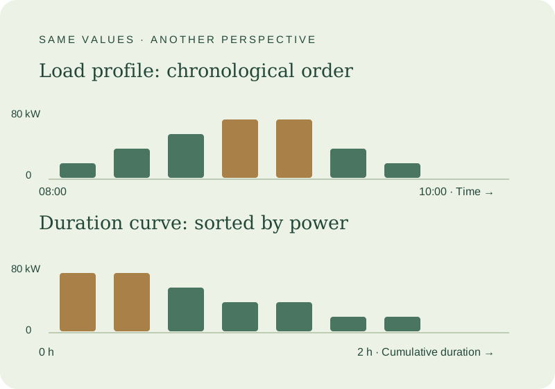
What is the difference between a load duration curve and a time series?
The load curve shows the measured values in chronological order: Monday morning follows Sunday night. High power levels are on the left of the duration curve, low levels on the right. The vertical axis represents kilowatts; the horizontal axis counts the corresponding hours.
The Fraunhofer project ProEnergie describes annual load duration curves, time series, grid representations, and peak load analysis as different views of the same energy data. Each answers a different question. For operational purposes, this means: first, identify how frequently high loads occur; then, examine the time series to determine when and under what conditions they arose. Fraunhofer Methods Overview.
"Annual duration curve" is the appropriate term for a period of one year. A monthly data set initially yields a monthly duration curve. Its shape cannot be extrapolated to the entire year without additional assumptions.
Different order, same energy
20 → 40 → 60 → 80 → 80 → 40 → 20 → 0 kW
80 → 80 → 60 → 40 → 40 → 20 → 20 → 0 kW
Define the data basis
For example, select the grid electricity import of a delivery point for a full calendar year. A system submeter and a feed-in measurement each describe something different. Record the time period, measurement direction, and data coverage alongside the evaluation.
We use average power values in kW for equal quarter-hours. If energy quantities are given in kWh per quarter-hour, the following applies: Power = Interval Energy / 0.25 hours. A cumulative meter reading is not an interval energy quantity. Information on units, timestamps, and data status can be found in our Guide to Load Profile Data Verification.
Keep the original time series. Sort a working copy that keeps each reading with its interval duration. Otherwise, you lose the link between the power level and what was happening in your business.
Creating a load duration curve step by step
Our own synthetic model, no customer load profile: Eight complete quarter-hours from 08:00 to 10:00 on January 15, 2026, chronologically contain the following power values: 20, 40, 60, 80, 80, 40, 20 and 0 kW . Each value is considered the average of its entire interval.
- Sort the eight complete records by power, highest first.
- Continue assigning each item its duration of 0.25 hours.
- Add these durations from left to right.
- For each value, draw a horizontal line segment representing its interval duration. This ensures that the area calculation remains unambiguous.
| Power | Number of quarter hours | Duration of this level | Total duration at the end of the section | energy |
|---|---|---|---|---|
| 80 kW | 2 | 0.50 h | 0.50 h | 40 kWh |
| 60 kW | 1 | 0.25 h | 0.75 h | 15 kWh |
| 40 kW | 2 | 0.50 h | 1.25 h | 20 kWh |
| 20 kW | 2 | 0.50 h | 1.75 h | 10 kWh |
| 0 kW | 1 | 0.25 h | 2.00 h | 0 kWh |
| Total | 8 | 2.00 h | — | 85 kWh |
Move the table sideways if needed →
The calculation is: Energy = Sum of Power × Interval Duration. In this case: 40 + 15 + 20 + 10 = 85 kWh. Sorting does not change this sum or the recorded two hours. The average power is 85 kWh / 2 h = 42.5 kW.
Quarter-hours with at least 60 kW ( interval average ) comprise a total of 0.75 hours: 37.5 percent of the recorded time. Quarter-hours with more than 60 kW (interval average), on the other hand, comprise only 0.50 hours. This is not a measurement accurate to the second. The three quarter-hours do not have to follow each other directly in the original load profile.
60 kW: distinguishing between "at least" and "more than".
The value of exactly 60 kW provides the additional quarter of an hour at "at least".
Addressing different intervals and data gaps
With varying interval lengths, the number of measurements is insufficient. A 60-minute value is assigned four times the width of a 15-minute value. For example: 80 kW for 0.25 hours, 40 kW for 0.50 hours, and 20 kW for one hour together result in 1.75 hours and 60 kWh. After sorting, the actual durations are cumulatively calculated. Unweighted counting would distort the proportions.
However, a larger interval between timestamps does not necessarily prove a longer measurement duration: It could indicate a data gap. The export description must clarify this. Use a confirmed, uniform measurement grid in the compass; sections with varying grids will be imported separately.
Distinguishing between zero and gap
A missing quarter-hour is neither counted as zero nor silently extended. If the 60 kW value is missing from the model, 70 kWh over 1.75 recorded hours remain. The total consumption over the full two hours is then unknown. A confirmed zero value, however, counts as observed time. The SMARD manual also distinguishes complete aggregations from missing data. Federal Network Agency: data processing and time specifications.
Zero is a measured value. A gap remains unknown.
All eight intervals are recorded.
- 20
- 40
- 60
- 80
- 80
- 40
- 20
- 0
Values in kW · each slot corresponds to 15 minutes
0 kW × 0.25 h = 0 kWh
The quarter hour counts towards the recorded time.
The third measurement is unknown.
- 20
- 40
- ?
- 80
- 80
- 40
- 20
- 0
Same target period – the gap remains visible
? kW × 0.25 h = ? kWh
The energy over the full 2.00 h is unknown.
Correctly account for daylight saving time and year length
In German local time, one hour is missing in spring; in autumn, one hour occurs twice. This in itself is not a data error. Unique UTC timestamps or appropriate UTC offsets distinguish the two autumn hours. They must not be deleted as supposed duplicates. Federal Network Agency: Time change in measurement time series.
Check the expected amount of data
A full normal calendar year comprises 8,760 hours, a leap year 8,784 hours. For complete quarter-hour series, this corresponds to 35,040 and 35,136 intervals, respectively. These figures serve as a completeness check, not a requirement for an incomplete curve. Your time axis may only contain the intervals actually evaluated; The target period and coverage belong alongside it.
Distinguish between duration, operating time, and usage hours
Our model includes two recorded hours and 1.75 hours of positive grid electricity import. This does not imply a specific machine runtime: Multiple systems, standby consumption, or on-site generation could be connected to the shared meter.
The calculated usage hours based on the measured maximum are, in this example, 85 kWh / 80 kW = 1.0625 hours. This answers a hypothetical question: How long would this maximum have to remain constant to account for the same amount of energy? It does not tell us how long the system was actually operating at 80 kW.
Specify the reference power
When calculating plant full-load hours, the rated power is often used as the reference power. It must be explicitly stated and cannot simply be replaced by the measured maximum. The Bavarian State Office for the Environment explains that full-load hours also include partial-load hours converted to full load. LfU: Operating and full-load hours.

Using the compass to find the right next question
After analysing a suitable measurement series, you can select the Load Profile Compass view called “load duration curve”. It shows interval power values sorted in descending order over recorded hours. Check the period and coverage. To examine particular times, switch back to the chronological view or heat map.
Two completely different shift sequences can produce the same duration curve. Similarly, spot costs can only be calculated if consumption and price are combined for the same delivery interval. Sorted power alone is not sufficient. Storage capacity also cannot be determined solely from the curve: consecutive peak periods, charging opportunities, and technical limitations remain crucial.
For billing issues, the next step involves looking at peak loads and RLM network charges . For procurement issues, Hasan Sahin and the energy team consider the original load profile along with operating times, planned changes, and the contract period.
Which representation leads to the answer?
How often is power demand high?
Interval power + respective duration
Load Duration Curve
In the model: at least 60 kW over a total of 0.75 h.
When does peak demand occur in your business?
Original timestamp + operational information
Time history, heat map if required
The sorting does not include times or shift sequences.
What are the spot costs?
Amount of energy + price of the same delivery interval
Time-aligned cost calculation
Without the appropriate temporal allocation, the basis for calculation is missing.
What storage size is suitable?
Peak sequence + charging opportunities + technical limits
Analysis of the chronological measurement series
A duration curve alone does not determine storage size.
Frequently Asked Questions
Can I create an annual duration curve myself in a table?
Yes. Sort a working copy by power and add the total interval durations. Energy and recorded time must match before and after sorting.
Does the right edge show the avoidable base load?
It shows low measured power levels. Additional operational information is needed to determine whether these reflect essential operation, standby or consumption that can be adjusted.
How should I handle negative power values?
First, clarify the measurement convention. Negative values can represent, for example, the opposite direction of flow. Maintain the sign and consider positive and negative energy quantities separately.
Is a short file sufficient for an annual forecast?
No. A short duration curve describes the recorded time. Seasonality, capacity utilization, downtime, and new installations can alter the rest of the year. Extrapolating data requires its own verifiable assumptions.